Brief Overview - How to use the MVG library
Introduction
The MultiViz Analytics Engine (MVG) Library is a Python library that enables the use of Viking Analytics’s MVG Analytics Service. To access this service, Viking Analytics (VA) provides a REST API towards its analytics server. The simplification of access to this service is enabled by the VA-MVG Python package, which allows interaction with the service via regular python calls.
This interactive document shall show the whole flow working with the service from Python, from data upload to retrieval of analysis results for the analysis of vibration signals.
Signing up for the service
For commercial use of the service, you will need to acquire a token from Viking Analytics. For the example here, we use a built-in token for demo. Please contact us for a free trial and provide you with your token.
Python Pre-requisites
Make sure you have Python 3.6 or higher installed.
In the following section we will walk through the code needed for the API interaction
Imports
First, we begin with the general imports of Python libraries that are needed as part of this project.
[1]:
import json
import os
import sys
from pathlib import Path

import pandas as pd
We proceed by installing the MVG library in our project.
[ ]:
!{sys.executable} -m pip install va-mvg
We follow by importing the MVG library.
The library documentation is available at https://vikinganalytics.github.io/mvg/index.html.
[2]:
from mvg import MVG
from mvg.exceptions import MVGAPIError
We begin by instantiating a “session” object with the MVG library. A session object basically caches the endpoint and the token, to simplify the calls to the MVG library.
Note
Each TOKEN is used for Authorization AND Authentication. Thus, each unique token represents a unique user, each user has it own, unique database on the VA-MVG’ service.
You need to insert your token received from Viking Analytics here: Just replace "os.environ['TEST_TOKEN']" by your token as a string.
[3]:
ENDPOINT = "https://api.beta.multiviz.com"
# Replace by your own Token
VALID_TOKEN = os.environ['TEST_TOKEN']
[4]:
session = MVG(ENDPOINT, VALID_TOKEN)
We now check if the server is alive. The hello message contains the API version:
[5]:
session.say_hello()
[5]:
{'name': 'MultiViz Engine API',
 'version': 'v0.3.2',
 'swagger': 'http://api.beta.multiviz.com/docs'}
Sources and Measurements
Before we begin, we will ensure there are no previously existing sources and if there are, we will delete them.
[7]:
sources = session.list_sources()

for src in sources:
    print(f"Deleting {src['source_id']}")
    session.delete_source(src['source_id'])
Deleting iris
Deleting u0001
Deleting u0002
Deleting u0003
Deleting u0004
Deleting u0005
Deleting u0006
The example below revolves around a source with source_id “u0001”.
For convenience, this source and its measurements are available with the package distribution.
You can retrieve the data from our public charlie repo https://github.com/vikinganalytics/va-data-charlie.git
[ ]:
!git clone --depth=1 https://github.com/vikinganalytics/va-data-charlie.git
[6]:
# Path to the source folder
REF_DB_PATH = Path.cwd() / "va-data-charlie" / "charlieDb" / "acc"
# Definition of the source_id
SOURCE_ID = "u0001"
Creating a Source
A source represents a vibration data source, typically a vibration sensor. Internally, in the analytics engine and data storage, all vibration data is stored under its source. In essence, a source is an identifier formed by
the source ID
metadata with required fields
optional arbitrary customer specific ‘free form’ data belonging to the source
channel definition as a list
The vibration service will only rely on the required fields. The free form data is a possibility for the client side to keep together source information, measurements and metadata which may be interesting for the analytics built-in features in the service. Examples of the free form data include location of sensor or the name of the asset which is mounted on. As we will see later, timestamps are internally represented as milliseconds since EPOCH (Jan 1st 1970), for that reason it is good practice to include the timezone where the measurement originated in the metadata. In addition, we provide the channel definition that contains the waveform data. Each channel represents a waveform. Thus, if the sensor only have one channel, we need to provide only the name given to the raw waveform for that channel. If the sensor has two or more channels, like ina tri-axial sensor, one needs to provide the name of the channels corresponding to the different waveforms that will be available in the measurements.
[9]:
meta_information = {'assetId': 'assetJ', 'measPoint': 'mloc01', 'location': 'cancun', 'timezone': 'Europe/Stockholm'}
session.create_source(SOURCE_ID, meta=meta_information, channels=["acc"])
session.get_source(SOURCE_ID)
[9]:
{'source_id': 'u0001',
 'meta': {'assetId': 'assetJ',
  'measPoint': 'mloc01',
  'location': 'cancun',
  'timezone': 'Europe/Stockholm'},
 'properties': {'data_class': 'waveform', 'channels': ['acc']}}
List sources
We can now check if our source actually has been created, by listing all the sources in the database. This function provides all the existing information about the source. Notice how in the source properties, one can see that the type of data to be uploaded for the source will be a waveform given that when one passes a channel definition to the source. The server interprets this as expecting for each measurement to be waveform data with the names of channels listed by the channel variable.
[10]:
session.list_sources()
[10]:
[{'source_id': 'u0001',
  'meta': {'assetId': 'assetJ',
   'measPoint': 'mloc01',
   'location': 'cancun',
   'timezone': 'Europe/Stockholm'},
  'properties': {'data_class': 'waveform', 'channels': ['acc']}}]
Uploading Measurements
Now that we have created a source, we can upload vibration measurements related to the source. The information needed to create a measurement consists of
sid: name of the source ID to associate the measurement with a source.
duration: float value that represent the duration, in seconds, of the measurement to estimate the sampling frequency.
timestamp: integer representing the milliseconds since EPOCH of when the measurement was taken.
data: list of floating point values representing the raw data of the vibration measurement.
meta: additional meta information for later use by the client but not to be processed by the analytics engine.
In this example, all the measurement data is stored as csv and json files, where the timestamp is the name of each of these files. On the csv file, the header of the colum of data corresponds to the channel name.
[11]:
# meas is a list of timestamps representing the measurements in our repo
src_path = REF_DB_PATH / SOURCE_ID
meas = [f.stem for f in Path(src_path).glob("*.csv")]
[12]:
# We iterate over all of elements in this list
for m in meas:

    # raw data per measurement
    TS_MEAS_FILE = str(m) + ".csv"  # filename
    TS_MEAS = REF_DB_PATH / SOURCE_ID / TS_MEAS_FILE  # path to file
    ts_df = pd.read_csv(TS_MEAS)  # read csv into df
    accs = ts_df.iloc[:, 0].tolist()  # convert to list
    print(f"Read {len(ts_df)} samples")

    # meta information file per measurement
    TS_META_FILE = str(m) + ".json"  # filename
    TS_META = REF_DB_PATH / SOURCE_ID / TS_META_FILE  # path
    with open(TS_META, "r") as json_file:  # read json
        meas_info = json.load(json_file)  # into dict
    print(f"Read meta:{meas_info}")

    # get duration and other meta info
    duration = meas_info['duration']
    meta_info = meas_info['meta']

    # Upload measurements
    print(f"Uploading {TS_MEAS_FILE}")
    try:
        session.create_measurement(sid=SOURCE_ID,
                                   duration=duration,
                                   timestamp=int(m),
                                   data={"acc": accs},
                                   meta=meta_info)
    except MVGAPIError as exc:
        print(str(exc))
Read 40000 samples
Read meta:{'duration': 2.8672073400507907, 'meta': {}}
Uploading 1570186860.csv
Read 40000 samples
Read meta:{'duration': 2.8672073400507907, 'meta': {}}
Uploading 1570273260.csv
Read 40000 samples
Read meta:{'duration': 2.8672073400507907, 'meta': {}}
Uploading 1570359660.csv
Read 40000 samples
Read meta:{'duration': 2.8672073400507907, 'meta': {}}
Uploading 1570446060.csv
Read 40000 samples
Read meta:{'duration': 2.8672073400507907, 'meta': {}}
Uploading 1570532460.csv
Read 40000 samples
Read meta:{'duration': 2.8672073400507907, 'meta': {}}
Uploading 1570618860.csv
Read 40000 samples
Read meta:{'duration': 2.8672073400507907, 'meta': {}}
Uploading 1570705260.csv
Read 40000 samples
Read meta:{'duration': 2.8672073400507907, 'meta': {}}
Uploading 1570791660.csv
Read 40000 samples
Read meta:{'duration': 2.8672073400507907, 'meta': {}}
Uploading 1570878060.csv
Read 40000 samples
Read meta:{'duration': 2.8672073400507907, 'meta': {}}
Uploading 1570964460.csv
Read 40000 samples
Read meta:{'duration': 2.8672073400507907, 'meta': {}}
Uploading 1571050860.csv
Read 40000 samples
Read meta:{'duration': 2.8672073400507907, 'meta': {}}
Uploading 1571137260.csv
Read 40000 samples
Read meta:{'duration': 2.8672073400507907, 'meta': {}}
Uploading 1571223660.csv
Read 40000 samples
Read meta:{'duration': 2.8672073400507907, 'meta': {}}
Uploading 1571310060.csv
Read 40000 samples
Read meta:{'duration': 2.8672073400507907, 'meta': {}}
Uploading 1571396460.csv
Read 40000 samples
Read meta:{'duration': 2.8672073400507907, 'meta': {}}
Uploading 1571482860.csv
Read 40000 samples
Read meta:{'duration': 2.8672073400507907, 'meta': {}}
Uploading 1571569260.csv
Read 40000 samples
Read meta:{'duration': 2.8672073400507907, 'meta': {}}
Uploading 1571655660.csv
Read 40000 samples
Read meta:{'duration': 2.8672073400507907, 'meta': {}}
Uploading 1571742060.csv
Read 40000 samples
Read meta:{'duration': 2.8672073400507907, 'meta': {}}
Uploading 1571828460.csv
Read 40000 samples
Read meta:{'duration': 2.8672073400507907, 'meta': {}}
Uploading 1571914860.csv
Read 40000 samples
Read meta:{'duration': 2.8672073400507907, 'meta': {}}
Uploading 1572001260.csv
Read 40000 samples
Read meta:{'duration': 2.8672073400507907, 'meta': {}}
Uploading 1572087660.csv
Read 40000 samples
Read meta:{'duration': 2.8672073400507907, 'meta': {}}
Uploading 1572177660.csv
Read 40000 samples
Read meta:{'duration': 2.8672073400507907, 'meta': {}}
Uploading 1572264060.csv
Read 40000 samples
Read meta:{'duration': 2.8672073400507907, 'meta': {}}
Uploading 1572350460.csv
Read 40000 samples
Read meta:{'duration': 2.8672073400507907, 'meta': {}}
Uploading 1572436860.csv
Read 40000 samples
Read meta:{'duration': 2.8672073400507907, 'meta': {}}
Uploading 1572523260.csv
Read 40000 samples
Read meta:{'duration': 2.8672073400507907, 'meta': {}}
Uploading 1572609660.csv
Read 40000 samples
Read meta:{'duration': 2.8672073400507907, 'meta': {}}
Uploading 1572696060.csv
Read 40000 samples
Read meta:{'duration': 2.8672073400507907, 'meta': {}}
Uploading 1572782460.csv
Read 40000 samples
Read meta:{'duration': 2.8672073400507907, 'meta': {}}
Uploading 1572868860.csv
Read 40000 samples
Read meta:{'duration': 2.8672073400507907, 'meta': {}}
Uploading 1572955260.csv
Read 40000 samples
Read meta:{'duration': 2.8672073400507907, 'meta': {}}
Uploading 1573041660.csv
Read 40000 samples
Read meta:{'duration': 2.8672073400507907, 'meta': {}}
Uploading 1573128060.csv
Read 40000 samples
Read meta:{'duration': 2.8672073400507907, 'meta': {}}
Uploading 1573214460.csv
Read 40000 samples
Read meta:{'duration': 2.8672073400507907, 'meta': {}}
Uploading 1573300860.csv
Read 40000 samples
Read meta:{'duration': 2.8672073400507907, 'meta': {}}
Uploading 1573387260.csv
Read 40000 samples
Read meta:{'duration': 2.8672073400507907, 'meta': {}}
Uploading 1573473660.csv
Read 40000 samples
Read meta:{'duration': 2.8672073400507907, 'meta': {}}
Uploading 1573560060.csv
Read 40000 samples
Read meta:{'duration': 2.8672073400507907, 'meta': {}}
Uploading 1573646460.csv
Read 40000 samples
Read meta:{'duration': 2.8672073400507907, 'meta': {}}
Uploading 1573732860.csv
Read 40000 samples
Read meta:{'duration': 2.8672073400507907, 'meta': {}}
Uploading 1573819260.csv
Read 40000 samples
Read meta:{'duration': 2.8672073400507907, 'meta': {}}
Uploading 1573905660.csv
Read 40000 samples
Read meta:{'duration': 2.8672073400507907, 'meta': {}}
Uploading 1573992060.csv
Read 40000 samples
Read meta:{'duration': 2.8672073400507907, 'meta': {}}
Uploading 1574078460.csv
Read 40000 samples
Read meta:{'duration': 2.8672073400507907, 'meta': {}}
Uploading 1574164860.csv
Read 40000 samples
Read meta:{'duration': 2.8672073400507907, 'meta': {}}
Uploading 1574251260.csv
Read 40000 samples
Read meta:{'duration': 2.8672073400507907, 'meta': {}}
Uploading 1574337660.csv
Read 40000 samples
Read meta:{'duration': 2.8672073400507907, 'meta': {}}
Uploading 1574424060.csv
Check if we actually created the measurements by reading them.
[13]:
measurements = session.list_measurements(SOURCE_ID)
print(f"Read {len(measurements)} stored measurements")
Read 50 stored measurements
Analysis
We begin by listing all the features available in the service.
[14]:
available_features = session.supported_features()
available_features
[14]:
{'RMS': '1.0.0',
 'ModeId': '0.1.1',
 'BlackSheep': '1.0.0',
 'KPIDemo': '1.0.0',
 'ApplyModel': '0.1.0',
 'LabelPropagation': '0.1.0'}
In this example, we will show how to request the KPIDemo and ModeId features to be applied to the previously defined SOURCE_ID. The BlackSheep feature is aimed to population analytics. You can read about how to use it in the “Analysis and Results Visualization” example.
We will begin with the KPIDemo feature, which provides KPIs, such as RMS, for each vibration measurement. We proceed to request the analysis to the MVG service.
[46]:
KPI_u0001 = session.request_analysis(SOURCE_ID, 'KPIDemo')
KPI_u0001
[46]:
{'request_id': '9fa506fd651f10b05401840edf9f33cb', 'request_status': 'queued'}
The requested analysis will return a dictionary object with two elements. The first element is a "request_id" that can be used to retrieve the results after. The second element is "request_status" that provides the status right after placing the analysis request.
Before we are able to get the analysis results, we need to wait until those results are successfully completed.
We can query for the status of our requested analysis. The possible status are:
Queued: The analysis has not started in the remote server and it is in the queue to begin.
Ongoing: The analysis is been processed at this time.
Failed: The analysis is complete and failed to produce a result.
Successful: The analysis is complete and it produced a successful result.
[8]:
REQUEST_ID_KPI_u0001 = KPI_u0001['request_id']
status = session.get_analysis_status(REQUEST_ID_KPI_u0001)
print(f"KPI Analysis: {status}")
KPI Analysis: successful
The next feature is ModeId. The ‘ModeId’ feature displays all the operating modes over time of an individual asset. The similar procedure is repeated to request the analysis of the “ModeId” feature for our source “u0001”.
[29]:
ModeId_u0001 = session.request_analysis(SOURCE_ID, 'ModeId')
ModeId_u0001
[29]:
{'request_id': 'c2d48d6d59c317c39469d3eaade7de96', 'request_status': 'queued'}
We also check the status for our second feature.
[7]:
REQUEST_ID_ModeId_u0001 = ModeId_u0001['request_id']
status = session.get_analysis_status(REQUEST_ID_ModeId_u0001)
print(f"ModeId Analysis: {status}")
ModeId Analysis: successful
We can proceed to get the results by calling the corresponding requestIds for the feature of each source.
The output of the "get_analysis_results" function is a dictionary and we show the keys of one those dictionaries. The keys are the same for all features and contains seven elements. These elements are:
"status"indicates if the analysis was successful."request_id"is the identifier of the requested analysis."feature"is the name of the requested feature."results"includes the numeric results."inputs"includes the input information for the request analysis."error_info"includes the error information in case the analysis fails and it is empty if the analysis is successful."debug_info"includes debuging (log) information related to the failed analysis.
[31]:
session.wait_for_analyses([REQUEST_ID_ModeId_u0001, REQUEST_ID_KPI_u0001])
kpi_results = session.get_analysis_results(request_id=REQUEST_ID_KPI_u0001)
mode_results = session.get_analysis_results(request_id=REQUEST_ID_ModeId_u0001)

kpi_results.keys()
[31]:
dict_keys(['status', 'request_id', 'feature', 'results', 'inputs', 'error_info', 'debug_info'])
Visualization
The MVG Library incorporates a module that facilitates the handling of the results and its visualization. Using this module, it becomes easier to convert the results into a Pandas dataframe for ease of manipulation. In addition, it enables to quickly evaluate the results by getting a summary of them or visualize them.
The name of this module is "analysis_classes" and we begin by calling it.
[9]:
from mvg import analysis_classes
The first step requires parsing the results available from the analysis. We begin by showing how to do this with the KPIDemo feature.
[10]:
kpi_results_parsed = analysis_classes.parse_results(kpi_results)
From here, we can call these results into a Pandas dataframe.
[11]:
df_kpi = kpi_results_parsed.to_df()
df_kpi.head()
[11]:
| timestamps | rms_acc | peak_acc | peak2peak_acc | variance_acc | crest_factor_acc | utilization_acc | dc_component_acc | datetime | |
|---|---|---|---|---|---|---|---|---|---|
| 0 | 1570186860 | 0.647086 | 2.686563 | 5.313293 | 0.418720 | 4.151786 | 1 | -0.140237 | 2019-10-04 11:01:00+00:00 |
| 1 | 1570273260 | 0.647123 | 2.691750 | 5.367004 | 0.418769 | 4.159563 | 1 | -0.140420 | 2019-10-05 11:01:00+00:00 |
| 2 | 1570359660 | 0.646619 | 2.715251 | 5.414856 | 0.418116 | 4.199152 | 1 | -0.140239 | 2019-10-06 11:01:00+00:00 |
| 3 | 1570446060 | 0.646873 | 2.685147 | 5.351562 | 0.418445 | 4.150966 | 1 | -0.140347 | 2019-10-07 11:01:00+00:00 |
| 4 | 1570532460 | 0.646643 | 2.726605 | 5.395325 | 0.418147 | 4.216556 | 1 | -0.140423 | 2019-10-08 11:01:00+00:00 |
From the results, we can see that the KPIDemo feature provides some KPIs, e.g. rms and peak-to-peak. All this is available for each measurement.
We can request to display a summary of the results.
[12]:
kpi_results_parsed.summary()
=== KPIDemo ===
request_id 9fa506fd651f10b05401840edf9f33cb
from 20191004-11:01.00 to 20191122-12:01.00

+-------+--------------+------------+------------+-----------------+----------------+--------------------+-------------------+--------------------+
|       |   timestamps |    rms_acc |   peak_acc |   peak2peak_acc |   variance_acc |   crest_factor_acc |   utilization_acc |   dc_component_acc |
|-------+--------------+------------+------------+-----------------+----------------+--------------------+-------------------+--------------------|
| count | 50           | 50         |  50        |       50        |     50         |          50        |                50 |         50         |
| mean  |  1.57231e+09 |  0.611691  |   2.81764  |        5.40059  |      0.377299  |           4.62976  |                 1 |         -0.120874  |
| std   |  1.26105e+06 |  0.0565414 |   0.278079 |        0.378225 |      0.0636172 |           0.333367 |                 0 |          0.0141936 |
| min   |  1.57019e+09 |  0.484564  |   2.26056  |        4.55438  |      0.234802  |           4.12339  |                 1 |         -0.140524  |
| 25%   |  1.57125e+09 |  0.627912  |   2.68338  |        5.31364  |      0.394273  |           4.20402  |                 1 |         -0.140196  |
| 50%   |  1.57231e+09 |  0.628307  |   2.84999  |        5.52634  |      0.39477   |           4.80641  |                 1 |         -0.112316  |
| 75%   |  1.57337e+09 |  0.64684   |   3.06661  |        5.69377  |      0.418402  |           4.89065  |                 1 |         -0.10966   |
| max   |  1.57442e+09 |  0.647694  |   3.13609  |        5.79639  |      0.419507  |           4.99256  |                 1 |         -0.109065  |
+-------+--------------+------------+------------+-----------------+----------------+--------------------+-------------------+--------------------+
[12]:
| timestamps | rms_acc | peak_acc | peak2peak_acc | variance_acc | crest_factor_acc | utilization_acc | dc_component_acc | |
|---|---|---|---|---|---|---|---|---|
| count | 5.000000e+01 | 50.000000 | 50.000000 | 50.000000 | 50.000000 | 50.000000 | 50.0 | 50.000000 |
| mean | 1.572306e+09 | 0.611691 | 2.817641 | 5.400591 | 0.377299 | 4.629763 | 1.0 | -0.120874 |
| std | 1.261051e+06 | 0.056541 | 0.278079 | 0.378225 | 0.063617 | 0.333367 | 0.0 | 0.014194 |
| min | 1.570187e+09 | 0.484564 | 2.260560 | 4.554382 | 0.234802 | 4.123387 | 1.0 | -0.140524 |
| 25% | 1.571245e+09 | 0.627912 | 2.683375 | 5.313644 | 0.394273 | 4.204021 | 1.0 | -0.140196 |
| 50% | 1.572307e+09 | 0.628307 | 2.849990 | 5.526337 | 0.394770 | 4.806408 | 1.0 | -0.112316 |
| 75% | 1.573366e+09 | 0.646840 | 3.066612 | 5.693771 | 0.418402 | 4.890653 | 1.0 | -0.109660 |
| max | 1.574424e+09 | 0.647694 | 3.136087 | 5.796387 | 0.419507 | 4.992559 | 1.0 | -0.109065 |
Finally, we can generate a plot that displays these results. When plotting the results for the KPIDemo feature, one selects the KPI to be displayed by passing the parameter "kpi". If this parameter is not included, the plot function will display the results of the first column in the summary dataframe after the timestamps, which is the RMS value.
[14]:
kpi_results_parsed.plot()
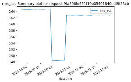
[14]:
''
All these functions are available for the ModeId feature as well. We proceed to repeat the same procedure for this other feature.
We begin by parsing the results. In this particular case, we need to define the unit of time to perform the epoch conversion to datetime. The default unit is milliseconds, but we use seconds here as the timestamps for this source is based on seconds. The timezone can also be defined, to increase the precision of these results.
[38]:
mode_results_parsed = analysis_classes.parse_results(mode_results, t_unit="s")
First, we generate the pandas dataframe of ModeId results.
[39]:
df_mode = mode_results_parsed.to_df()
df_mode.head()
[39]:
| timestamps | labels | uncertain | mode_probability | datetime | |
|---|---|---|---|---|---|
| 0 | 1570186860 | 0 | False | 0.912743 | 2019-10-04 11:01:00+00:00 |
| 1 | 1570273260 | 0 | False | 0.972841 | 2019-10-05 11:01:00+00:00 |
| 2 | 1570359660 | 0 | False | 0.929741 | 2019-10-06 11:01:00+00:00 |
| 3 | 1570446060 | 0 | False | 0.999620 | 2019-10-07 11:01:00+00:00 |
| 4 | 1570532460 | 0 | False | 0.978940 | 2019-10-08 11:01:00+00:00 |
From the results, we can see that the ModeId feature provides a mode label for each timestamp, together with a boolean describing the certainty around this mode label and its probability.
We can also request to display a summary of the results.
[40]:
mode_results_parsed.summary()
=== ModeId ===
request_id c2d48d6d59c317c39469d3eaade7de96
from 20191004-11:01.00 to 20191122-12:01.00

Labels
+----------+----------+-----------+--------------------+------------+
|   labels |   counts |   portion |   mode_probability |   datetime |
|----------+----------+-----------+--------------------+------------|
|        0 |       17 |        34 |                 17 |         17 |
|        1 |        8 |        16 |                  8 |          8 |
|        2 |       25 |        50 |                 25 |         25 |
+----------+----------+-----------+--------------------+------------+

Labels & uncertain labels
+------------+-----------+--------------------+------------+----------+
|            |   portion |   mode_probability |   datetime |   counts |
|------------+-----------+--------------------+------------+----------|
| (0, False) |        34 |                 17 |         17 |       17 |
| (1, False) |        16 |                  8 |          8 |        8 |
| (2, False) |        50 |                 25 |         25 |       25 |
+------------+-----------+--------------------+------------+----------+

Emerging Modes
+----+---------+-----------------+-----------------+-------------------+---------------------------+
|    |   modes |   emerging_time |   max_prob_time |   max_probability | datetime                  |
|----+---------+-----------------+-----------------+-------------------+---------------------------|
|  0 |       0 |      1570186860 |      1570446060 |          0.99962  | 2019-10-04 11:01:00+00:00 |
|  1 |       1 |      1571655660 |      1571742060 |          0.997126 | 2019-10-21 11:01:00+00:00 |
|  2 |       2 |      1572350460 |      1573041660 |          0.999948 | 2019-10-29 12:01:00+00:00 |
+----+---------+-----------------+-----------------+-------------------+---------------------------+
[40]:
[        counts  portion  mode_probability  datetime
 labels
 0           17     34.0              17.0        17
 1            8     16.0               8.0         8
 2           25     50.0              25.0        25,
                   portion  mode_probability  datetime  counts
 labels uncertain
 0      False         34.0              17.0        17      17
 1      False         16.0               8.0         8       8
 2      False         50.0              25.0        25      25,
    modes  emerging_time  max_prob_time  max_probability  \
 0      0     1570186860     1570446060         0.999620
 1      1     1571655660     1571742060         0.997126
 2      2     1572350460     1573041660         0.999948

                    datetime
 0 2019-10-04 11:01:00+00:00
 1 2019-10-21 11:01:00+00:00
 2 2019-10-29 12:01:00+00:00  ]
The summary of the results describes the number of timestamps for each mode and how many of these timestamps are uncertain. Uncertain areas appear as a gray rectangle above the corresponding periods in the modes plot.
In addition, it provides information on the emerging modes. Emerging modes describes the time (timestamp) each one of the modes first appeared. This information can be useful to identify if a new mode is affecting or appearing in the asset.
Finally, we can generate a plot that displays display the different modes over time.
[47]:
mode_results_parsed.plot()
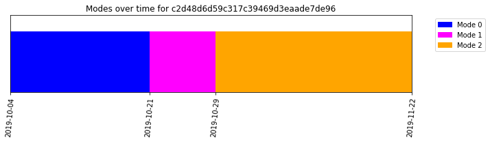
[47]:
''
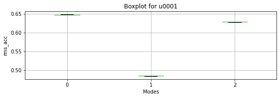
Lastly, we can combine the information from the KPIDemo and ModeId features to display a boxplot of the “RMS” for each one of the operating modes.
First, we merge the “KPI” and “ModeId” dataframes.
[48]:
df_u0001 =  pd.merge_asof(df_kpi, df_mode, on="timestamps")
df_u0001.head()
[48]:
| timestamps | rms_acc | peak_acc | peak2peak_acc | variance_acc | crest_factor_acc | utilization_acc | dc_component_acc | datetime_x | labels | uncertain | mode_probability | datetime_y | |
|---|---|---|---|---|---|---|---|---|---|---|---|---|---|
| 0 | 1570186860 | 0.647086 | 2.686563 | 5.313293 | 0.418720 | 4.151786 | 1 | -0.140237 | 2019-10-04 11:01:00+00:00 | 0 | False | 0.912743 | 2019-10-04 11:01:00+00:00 |
| 1 | 1570273260 | 0.647123 | 2.691750 | 5.367004 | 0.418769 | 4.159563 | 1 | -0.140420 | 2019-10-05 11:01:00+00:00 | 0 | False | 0.972841 | 2019-10-05 11:01:00+00:00 |
| 2 | 1570359660 | 0.646619 | 2.715251 | 5.414856 | 0.418116 | 4.199152 | 1 | -0.140239 | 2019-10-06 11:01:00+00:00 | 0 | False | 0.929741 | 2019-10-06 11:01:00+00:00 |
| 3 | 1570446060 | 0.646873 | 2.685147 | 5.351562 | 0.418445 | 4.150966 | 1 | -0.140347 | 2019-10-07 11:01:00+00:00 | 0 | False | 0.999620 | 2019-10-07 11:01:00+00:00 |
| 4 | 1570532460 | 0.646643 | 2.726605 | 5.395325 | 0.418147 | 4.216556 | 1 | -0.140423 | 2019-10-08 11:01:00+00:00 | 0 | False | 0.978940 | 2019-10-08 11:01:00+00:00 |
The MVG library provides additional visualization functions that can help towards this goal. Thus, we import the visualization module.
[49]:
from mvg import plotting
Now, we can proceed to plot the boxplot for the requested kpi.
[50]:
plotting.modes_boxplot(df_u0001, "rms_acc", SOURCE_ID)
[50]:
<AxesSubplot:title={'center':'Boxplot for u0001'}, xlabel='Modes', ylabel='rms_acc'>
Here we conclude our brief overview to begin using the MultiViz Analytics Engine (MVG) Library.