Working with Tabular Data
Although MVG has been designed with vibration waveform data in mind, it still works wonderfully well with non-vibration or KPI data. We refer to this as tabular timeseries data. Each measurement consists of one or more variables captured at the same time. This is different from the vibration waveform data, where each measurement is a short measurement sample from one vibration sensor.
In this example, we will show how to work with tabular sources and measurements, and how to create an analysis. If you have seen any of the previous examples, much of this one will be familiar to you.
Imports
Beyond importing MVG and the ModeId analysis class, we want to use pandas for loading and processing the data before the analysis.
[1]:
import os
from pprint import pprint
from pathlib import Path

import pandas as pd

from mvg import MVG
from mvg.analysis_classes import ModeId
After importing we create the MVG session that let us communicate with the MVG server. For that we need an endpoint URL and a valid token. If you do not have a token, you can get one here.
Note
Each token is used for Authorization AND Authentication. Thus, each unique token represents a unique user, each user has it own, unique database on the VA-MVG’ service.
You need to insert your token received from Viking Analytics here: Just replace "os.environ['TEST_TOKEN']" by your token as a string.
[2]:
ENDPOINT = "http://api.beta.multiviz.com"
TOKEN = os.environ['TEST_TOKEN']
[3]:
session = MVG(ENDPOINT, TOKEN)
We will use a dataset that is collected from a heat pump in the cellar of one of the employees at Viking Analytics. The data is available in this git repository. We clone the repository to get access it. If you don’t have git you can download the data from the link.
[4]:
!git clone https://github.com/vikinganalytics/tabular-example-data.git
Cloning into 'tabular-example-data'...
[5]:
data_path = Path.cwd() / "tabular-example-data" / "heatpump.csv"
data_df = pd.read_csv(data_path)
data_df.head()
[5]:
| timestamp | T_out | T_down | T_kitchen | WATT | T_up | T_brine_in | T_brine_out | T_cellar | |
|---|---|---|---|---|---|---|---|---|---|
| 0 | 2018-02-01T00:00:00Z | 1.976053 | 38.367181 | 20.512105 | 2.780167 | 40.028018 | 3.690000 | 2.068514 | 10.965206 |
| 1 | 2018-02-01T01:40:00Z | 2.380000 | 36.940000 | 20.190000 | 3.045333 | 39.060000 | 3.560000 | 1.991486 | 10.924431 |
| 2 | 2018-02-01T03:25:00Z | 2.211223 | 37.715920 | 20.190000 | 3.060000 | 39.840240 | 3.598392 | 1.961608 | 10.982982 |
| 3 | 2018-02-01T05:10:00Z | 1.964956 | 37.940000 | 20.250000 | 3.151579 | 40.023789 | 3.611330 | 2.068670 | 10.888049 |
| 4 | 2018-02-01T06:55:00Z | 0.349134 | 37.551293 | 20.406457 | 3.257167 | 39.856860 | 3.690000 | 2.120000 | 10.941380 |
We loaded the .csv file into a dataframe object and printed out the first five rows. The timestamp was read as string timestamps, but for the MVG API we need the timestamps to be in milliseconds since EPOCH. So we need to do some data wrangling in order to get it to the correct data type.
We can use the function pandas.to_datetime() to convert a column into datetime objects. Then we can convert the timestamps into integers, which will automatically get converted to nanoseconds since EPOCH. Then, when dividing by 1e6 we get the same time in milliseconds. We can see that the conversion was successful by printing the first five rows again.
[6]:
data_df["timestamp"] = pd.to_datetime(data_df["timestamp"]).astype("int64") // 1000000
data_df.head()
[6]:
| timestamp | T_out | T_down | T_kitchen | WATT | T_up | T_brine_in | T_brine_out | T_cellar | |
|---|---|---|---|---|---|---|---|---|---|
| 0 | 1517443200000 | 1.976053 | 38.367181 | 20.512105 | 2.780167 | 40.028018 | 3.690000 | 2.068514 | 10.965206 |
| 1 | 1517449200000 | 2.380000 | 36.940000 | 20.190000 | 3.045333 | 39.060000 | 3.560000 | 1.991486 | 10.924431 |
| 2 | 1517455500000 | 2.211223 | 37.715920 | 20.190000 | 3.060000 | 39.840240 | 3.598392 | 1.961608 | 10.982982 |
| 3 | 1517461800000 | 1.964956 | 37.940000 | 20.250000 | 3.151579 | 40.023789 | 3.611330 | 2.068670 | 10.888049 |
| 4 | 1517468100000 | 0.349134 | 37.551293 | 20.406457 | 3.257167 | 39.856860 | 3.690000 | 2.120000 | 10.941380 |
To upload the data to the API we need to convert the dataframe into a dictionary on the format {column: values}. Fortunately, dataframes have a method to do just that, called to_dict(). It has an argument for changing the orientation of the resulting dictionary. By using to_dict("list") we will get it on the correct format.
Note
The dictionary must have a "timestamp" key and at least one more column, corresponding to a tracked variable. The to_dict("list") method will not include the index, so it is important to have the timestamp as a column in the data and not as an index.
[7]:
data_dict = data_df.to_dict("list")
Now that the data has been converted to the correct format we are ready to create the source and upload some measurements. When creating a tabular source, you must define the columns that the data will contain ahead of time. This is to prevent arbitrary data to be uploaded to the source. Besides the columns argument, creating a tabular source works the exact same way as creating a waveform source.
[8]:
session.create_tabular_source(
    sid="heatpump",
    meta={"location": "Molnlycke"},
    columns=data_df.columns.tolist()
)
We can check that the source was created correctly by getting the source information.
[9]:
source = session.get_source("heatpump")
pprint(source)
{'meta': {'location': 'Molnlycke'},
 'properties': {'columns': ['T_out',
                            'T_down',
                            'T_kitchen',
                            'WATT',
                            'T_up',
                            'T_brine_in',
                            'T_brine_out',
                            'T_cellar'],
                'data_class': 'tabular'},
 'source_id': 'heatpump'}
Next, let’s upload the data we prepared to the source
[10]:
session.create_tabular_measurement(
    sid="heatpump",
    data=data_dict
)
Now that we have a source with measurements we can request an analysis of the data from the server. Requesting analyses for tabular data works the same way as it does for waveform data. Although not all features will work for tabular data. The KPIDemo feature for example will only work with waveform data. Another thing to keep in mind is that when requesting population analyses, all sources to be analyzed simultaneously must have the same data class.
For now, we will simply run the mode identification algorithm.
[11]:
response = session.request_analysis(
    sid="heatpump",
    feature="ModeId",
)
request_id = response["request_id"]
To make the results easier to work with we can load them into an analysis class. There exists one for each analysis feature. Once the analysis is completed and we have received the results, we can instatiate the analysis class with the results dictionary.
[12]:
session.wait_for_analyses([request_id])
results = session.get_analysis_results(request_id)
analysis = ModeId(results)
The analysis class makes it very convenient to view the results. Let’s use the ModeId.plot() method to get an overview of the results.
[13]:
analysis.plot()
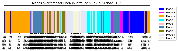
[13]:
''
The different modes help to identify between idle and have high-usage conditions along all seasons of the year.
When you are finished with the example you can go ahead and delete the source
[14]:
session.delete_source("heatpump")